Jose Manuel Echevarria Rubio

01Finding The Monk: The Webinar Recap

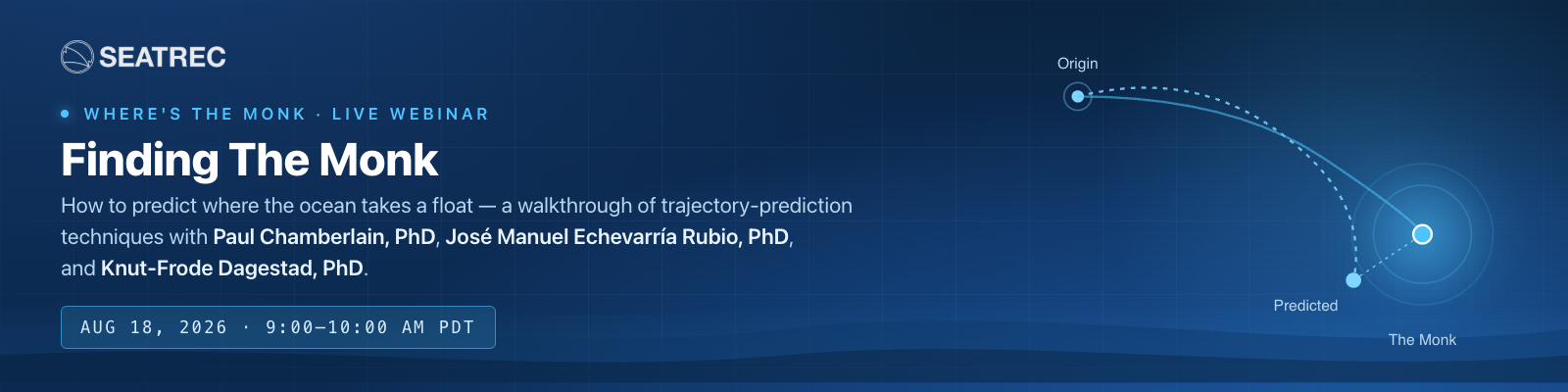
Last week Dr. Paul Chamberlain of Scripps Institution of Oceanography co-hosted a Seatrec webinar with the winners of our first two Where’s the Monk? trajectory-prediction contests, walking through the actual science — and, by their own admission, the actual luck — behind forecasting where a drifting ocean float will surface, days out, with no fresh GPS fix to correct against. If you missed our winner write-ups, catch up here: José Manuel Echevarría Rubio, Round 1 and Knut-Frode Dagestad, Round 2.

02The Challenge, Recapped

The Monk is an infiniTE float — Seatrec’s patented ocean-thermal-energy-harvesting profiler, out testing in the Atlantic and the Gulf of Mexico. Since deployment, it has logged more than 300 days at sea, completed over 700 dive profiles, and covered more than 7,000 kilometers, diving roughly every 11 hours down to an average parking depth near 900–960 meters before resurfacing just long enough to transmit its position.

Seatrec co-founder Yi Chao had the idea to turn that into a community challenge: give participants the float’s last confirmed GPS fix and its full historical track, then ask them to predict where it would resurface roughly nine days later — no peeking in between. The team named the float “the Monk,” partly for its solitary life at depth, and partly as a nod to oceanographer Walter Munk.

Round 1 drew 24 entrants; only four landed within 100 km of the true surfacing position, and José Manuel Echevarría Rubio won with an error of just 52 km, with an honorable mention to Ruoying (Roy) He and the Fathom Science team at North Carolina State University, whose prediction also landed within 100 km — along with two other entrants. Round 2 was a tighter finish: three predictions landed within 100 km, and Knut-Frode Dagestad of MET Norway took it by just 61 km, with honorable mentions to Liesvy Valladares Alfonso (CICIMAR-IPN) and Zach Dubroc (Mississippi Coding Academies).

03Why Is This So Hard? The Physics of a Growing Error Bar

Paul opened by framing the question everyone was really asking: if you drop something in the ocean and track it for a week, why is 50+ km of error the good outcome? His answer came down to where the uncertainty comes from — and it changes character over time:

• Early on (the “ballistic” regime): uncertainty grows roughly in proportion to time — small early errors in current velocity compound quickly.
• Later (the “diffusive” regime): uncertainty grows more slowly, in proportion to the square root of time, as the trajectory effectively randomizes.
• Over the longest horizons: any systematic bias in the ocean model re-asserts itself, and error growth goes linear again.

Layered on top of that: ocean models like Copernicus GLORYS product and NOAA’s HYCOM typically resolve currents only down to a handful of kilometers — but real ocean motion includes sub-mesoscale eddies, internal waves, and wind-driven variability at scales models simply can’t see. And because profiling floats spend most of their life at depth rather than at the surface, predicting them means resolving the full three-dimensional current field, not just what satellites can observe from above.

04Round 1: How José Manuel Won

José Manuel, a PhD candidate at CICIMAR-IPN studying sargassum transport in the Atlantic and Caribbean, adapted tools he already uses for tracking surface drifters to the Monk’s much deeper problem. Because the Monk spends more than 98% of its time below the surface, he built a three-phase dive model — roughly 30 minutes at the surface to transmit, a ~2.5 hour descent at 0.1 m/s, and around 7.5 hours parked near the deepest point of its dive (about 900 meters) — and sampled ocean currents at each phase separately, rather than assuming one depth for the whole trajectory. He discarded surface wind/wave (Stokes) drift entirely once testing confirmed it had no meaningful effect, since the float spends so little time at the surface.

Using Copernicus’s global Mercator current product (~9 km resolution, 8 depth levels) and OpenDrift for the simulation, he scored candidate configurations with the Liu–Weisberg skill score and ran a grid search (via scikit-learn) tuning a current “slip” coefficient and the length of the re-initialization window. His best setup — a 7-day reinitialization window and a current coefficient of 0.75 — produced a mean skill score of 0.96 across the float’s full 284-day history at the time (1.0 being a perfect match), and it’s what won him Round 1 with 52 km of error.

His own lessons learned: the vertical dive cycle matters as much as horizontal current speed, shorter reinitialization windows keep errors from compounding, and trustworthy skill metrics matter more than chasing any one lucky-looking result.

05Round 2: How Knut-Frode Won — and What His Colleague’s Research Adds

Knut-Frode, lead developer of OpenDrift, found the contest post on LinkedIn just two days before the Round 2 deadline and built his entry solo, in what he candidly called an “embarrassingly simplistic” version of José Manuel’s approach. He pulled the float’s historical track into Trajan (a standalone Python trajectory-analysis package originally built inside OpenDrift, now spun out so it can score any drift model’s output against observed tracks), then tested his simulation against the real historical positions. His first pass — surface currents only — performed poorly, as expected, since the Monk spends almost no time at the surface. His second pass, holding the float at a single eyeballed depth of 700 meters (versus José Manuel’s calculated ~900–960 meters), tracked the real trajectory far more closely, and that’s the current field he ultimately trusted for his forecast.

Rather than over-engineer it further, he made a judgment call: since forecast errors compound regardless of method, and Round 2 had fewer entrants than Round 1, the odds favored a good-enough model over a heavily-tuned one. He was open that part of this was a bet on variance:

His MET Norway colleague Jean Rabault joined to share related bias-correction research from an earlier DARPA ocean-prediction competition: combining multiple current products — satellite-derived (like Globcurrent) and model-based (Mercator, HYCOM, OSCAR) — with a simple linear regression outperformed any single product by 30–40% on the Liu–Weisberg skill score. A neural network trained on the same inputs didn’t beat the linear model, suggesting the individual products’ errors are already close to a fixed offset rather than a complex nonlinear relationship. On ensemble modeling more broadly: the best-performing ensemble member tends to stay best for only the next 1–2 days, but a bad member tends to stay bad for 7–10 days — making it more valuable to filter out consistently poor members than to chase the single best one.

06From the Q&A, and What’s Next

Is the deep ocean less chaotic than the surface?

Javier Zavala-Garay asked how dispersive currents are at 500–1,000 meters compared to the wind-driven surface layer. José Manuel’s view: deeper water masses are more thermally homogeneous and likely less stochastic than the surface mixed layer. Paul pointed to the DIMES experiment — which acoustically tracked floats in the Antarctic Circumpolar Current — as real-world evidence that meaningful current variability exists at depth too, even if it behaves differently than surface turbulence.

Could Lagrangian Coherent Structures help?

Sebastién Legrand raised the idea of using LCS/attractor analysis to flag when a trajectory is entering a region likely to bend a prediction off course. Knut-Frode had experimented with this before and wasn’t convinced it adds much beyond what a good drift simulation already captures — but was open to being wrong about it.

What’s the single easiest next improvement?

Both winners agreed: more complete dive-cycle metadata from Seatrec — exact time-at-surface and time-at-depth per dive — would sharpen everyone’s models. Yi Chao acknowledged that data exists but isn’t well surfaced today, and committed to publishing it more clearly for future rounds.

Looking ahead, Seatrec plans to run the Monk contest on a monthly cadence (weekly proved to be too much of a good thing), likely featuring a different float and location next round. Prizes escalate with repeat wins too — from a t-shirt, up to a jacket, up to a Seatrec cooler bag for anyone who takes the top spot three times. A well-earned congratulations to both winners — and a special shoutout to José Manuel, who successfully defended his PhD dissertation just two days after this session.