
Where's the Monk? Contest Webinar - Full Transcript
Where's the Monk? Contest Webinar — Full Transcript
Lightly edited for readability from the auto-generated recording transcript. For the recap with context, video, and slides, see Webinar on Finding the Monk Contest.
Welcome and Introduction
Paul Chamberlain: Good morning, everybody. Thanks so much for tuning in to the inaugural Where's the Monk contest seminar. Just to give you some background, this float was released in the Atlantic for testing purposes. Seatrec is always trying to improve their technology and make a more durable float that will last longer. Just as a side note, the Seatrec float has an energy-harvesting component to it, so it's actually generating positive energy in many parts of the world's ocean. So, hypothetically, these floats could last a very, very long time as they drift around in the ocean.
Yi (Chao) had this idea to focus the community on trajectory prediction, because that would be very useful for scientists — either to predict, or potentially to long-term navigate, where these Lagrangian drifters are going. So Yi had this great idea that we could create a contest where we would all compete to identify where this float is going to go. We all got together and brainstormed a name for the float. We came up with the Monk, because it's out in the middle of the ocean — very solitary, and it spends a lot of its time in rest and contemplation. But also, it's an homage to Walter Munk, a great oceanographer and somebody I personally have a lot of respect for.
So, the agenda for this presentation: first, our introduction and format. Then an overview of some common Lagrangian prediction frameworks and their error sources — and then, the highlight of this presentation, we have two titans of the Lagrangian prediction world, José Manuel Echevarría Rubio and Knut-Frode Dagestad, presenting on their work. And then we'll have questions and discussion.
First, I want to thank everybody for their participation. We are going to run this contest with some regularity, and continue to encourage participation with increasingly compelling prizes for winners, and we're hoping to have seminars to highlight these Lagrangian prediction techniques — and maybe even develop a publication on best practices.
So, with that, we'll get started. What I'm showing here is a plot of the first competition — the 24 applicants we received, and the errors of every one of the predictions. José Manuel Echevarría Rubio won with an error of 52 kilometers. Only four entrants had under 100 kilometers of error, and the question I want to tease apart is: why is it so hard to do this Lagrangian prediction? It seems like if you put something out in the ocean and waited a week, you'd have a better idea than 50 kilometers. Why does this distribution of uncertainty look like this?
The Physics of Trajectory Uncertainty
Paul Chamberlain: So we're going to go to a common description of the problem. We'll say that we're going to create an estimate of where the float is going to go — x is our state vector, where the float is, our GPS position. We integrate that from some time step to a future time step, using an estimate of the ocean velocity, which we'll call û (u-hat). If we integrate that forward, we get an estimate of the future position. Now, û is driven by an ocean model — or, since this is hopefully a blue-sky conversation, there are a lot of exotic methods we could employ: ensembles, AI, all kinds of things.
But just for the bread-and-butter Lagrangian prediction, we'll say this is an ocean model. The commonly used ones — and I'm genuinely interested to hear how the entrants approached this — I'd say the big three pillars of ocean modeling for Lagrangian particles are the Copernicus GLORYS (Global Ocean Reanalysis and Simulations) project, a large-scale physical ocean model; the HYCOM product, run by NOAA, another large-scale global model; and potentially some regional ocean models using the ROMS system.
If we build on this: error — the number we were looking at before, what we're trying to optimize against — equals the true location of the float minus our estimate. We can get the incremental error at every time step, and if we differentiate error with respect to time, we get an expression with two parts: the gradient of the estimated velocity times the existing error, plus a new model-error term that gets propagated into the system — the estimated velocity minus the true velocity. We'll call this new-model-error term η (eta). So η is basically how bad our velocity field is at each additional time step. This is a linearization of the uncertainty, and we can break η into two pieces: a model bias term, and η′ (eta-prime) — everything left over from a fundamental bias, defined critically by the fact that the expectation of η′ is zero. Think of η′ as high-frequency, unresolved physics not captured by a model grid cell — or as a catch-all for interpolation/representation error in how we integrate the Lagrangian prediction forward.
As for what η′ looks like in practice: there are some really good advection-scheme packages out there — OceanParcels, which I use; OpenDrift, which Knut-Frode Dagestad is the lead developer of; Octopus; TrackMass. This comes from a review paper by Van Sebille et al., 2018, which I read in preparing for this talk. These Lagrangian advection schemes use a variety of applied-math strategies — Runge-Kutta 4/5, Euler methods — each with trade-offs, and they're all freely and openly available, which is great for the community.
To explain why these different advection schemes matter: imagine a conceptual "true" ocean state with a lot of fine-scale complexity. Each path through that field represents a different advection scheme. A crude interpolation might jump between grid cells and produce a steppy trajectory; smarter interpolation smooths that out; a more advanced approach — spline interpolation, or a finer integrator time step — gives you yet another trajectory. The Van Sebille paper applies this in a real-world case, comparing several advection schemes to a theoretical solution, and the differences between them represent the uncertainty introduced by the advection scheme itself.
Going back to the bias and η′ terms: Lagrangian trajectories are nonlinear and path-dependent, so error from previous time steps propagates into the next and can confound results. For these ocean models, the exact state of the mesoscale eddy field defines the path — it's not enough to have the right energy spectrum on average; everything needs to be placed correctly, or you get the wrong answer, and these errors compound over time. A final wrinkle: profiling floats are doing exactly that — profiling up and down through the water column, experiencing ocean shear as they ascend and descend to park depth. Depending on the mission, a substantial percentage of displacement can happen at depth, so we need to resolve not just the two-dimensional placement of eddies, but the full three-dimensional current field — difficult, because most of our sampling comes from space-based remote sensing, which can't see beneath the surface. It's a strong argument for good profiling floats that can give you three-dimensional data about the ocean.
I don't know how AI is going to affect ocean modeling, but I do know it's improved my clip art — these images were generated with OpenAI. For sub-mesoscale processes: on the left is what a hypothetical model shows for ocean velocities — smooth, low resolution, because these models run at a global scale with finite processing power. The Copernicus and HYCOM models both run at a twelfth of a degree, so several kilometers to tens of kilometers is the scale we can resolve. In the real open ocean, there's a lot happening at much smaller scales — surface gravity waves, wind interaction, internal waves, currents — and many of these processes aren't resolved in models, or if they are, they're parameterized, and the parameterizations may not be fully robust. That's another source of uncertainty.
Going back to the math: η as a function of time is our bias plus η′. Our model error is the integral of η, and we can look at the autocovariance of the velocity error — call that c-sub-η — and integrate that to get the full model-error covariance. This was originally derived by G.I. Taylor in 1922, with a contemporary derivation along similar lines by LaCasce in 2008. Once you derive this term, on short timescales your uncertainty is proportional to time — the so-called ballistic regime, a term coined by Taylor. On long timescales, uncertainty is proportional to the square root of time — the dispersive regime.
Finally, if you have model bias — a constant bias term — integrating that gives you a bias timescale that's also proportional to time. So, breaking down why this prediction is so hard, why only four entrants got under 100 km of error: initially, after the float goes down into the water, we're in the ballistic regime, where uncertainty scales with time. As we leave that regime, we enter a diffusive regime, where uncertainty scales with the square root of time. And if there's bias in the model — which there likely is — over a long enough timescale we transition to model-bias-dominated uncertainty, proportional to time again. That's why, over a week, we get the uncertainties we do.
I'm genuinely curious to hear the methods people used to get the results they got, and I hope it encourages the community to adopt or refine them in future competitions. Some ideas for improving predictions: bespoke regional models with better interpolation/advection schemes or better representations of fine-scale motion (through parameterization or AI); ensemble forecasts, which is what I've been spending time on lately and find fairly effective; and using the float's full historical track to calibrate uncertainties from previous predictions.
But enough about my ideas — I think everyone's here to hear from the people who did this successfully. José, I'm sorry, I thought your last name was Rubio — I apologize, it should be José Echevarría. José is going first — we're all rooting for him, since he's about to defend his dissertation. José is a soon-to-be-minted PhD from CICIMAR-IPN in Mexico. [Editor's note: it's official — he's Dr. Echevarría Rubio, as of August 20, 2026.] José is an oceanographer and geospatial scientist who bridges marine science and data engineering. His research leverages satellite imagery, machine learning, and ocean transport modeling to track pelagic sargassum dynamics in the Atlantic and Caribbean. Before oceanography, he spent five years as an automation engineer designing embedded systems and data platforms, and he draws on those skills in his research. So, without further ado, I'll let José take it away.
Marta Bulaich: And if anyone has questions, feel free to put them in the chat or the Q&A.
Presentation: José Manuel Echevarría Rubio (Round 1 Winner)
José Manuel Echevarría Rubio: Thank you both for the introduction. Actually, Rubio is my second last name, so no problem.
Paul Chamberlain: Okay, all right.
José Manuel Echevarría Rubio: Let me share — can everyone see the presentation? Okay, hello everyone, and welcome to this section of the webinar on finding the Monk and how to predict where the ocean takes the float. My name is José Manuel. I'm a PhD candidate at CICIMAR, as Paul said, in La Paz, Baja California Sur, Mexico. I won the first contest of the Seatrec Challenge, and my forecast landed around 52 kilometers from the actual surfacing position of the float. Today I'll walk you through the modeling I did to make this possible.
Some background: in my PhD research I develop Lagrangian drift models — it's one of my research objectives — and here you can see a simulation I built for tracking pelagic sargassum detected by Sentinel-2 satellites as it drifts through the Caribbean and the Loop Current. In that case I used OpenDrift with Copernicus Marine currents, the GLORYS12 product. When Seatrec announced the contest, I saw the LinkedIn post and asked whether I could adapt what I do with in-situ drifter data and 2D surface advection to the Monk's much deeper, 3D problem.
Here's the challenge: Seatrec gave us the last confirmed GPS fix in June 2027. Our task was to predict where it would surface nine days later, on July 5, and it was located in the Gulf Stream. On the left you can see the full 184-day previous history of the float's track, and on the right, the official Seatrec portal where you can inspect the positions — latitude, longitude, and the depth of the profile at each coordinate. The first step was getting data for the forecast: I used the Copernicus Marine operational Mercator currents product, specifically the Global Analysis and Forecast, at 1/12 degree spatial resolution — about nine kilometers — and downloaded eight depth levels to build a currents cube covering the float's full mission, from deployment in the Gulf of Mexico to the final position.
I calculated the average depth of the profiles at around 961 meters, so the closest current layer, at 902 meters, was close enough to simulate advection in the deepest layer. I also tested adding surface (Stokes) drift for the time the float spent at the surface, but I discarded it — it didn't meaningfully impact the trajectory, since the float spends so little time above the wave base.
Here's the cube with the eight depth levels built from Copernicus Marine — the closest layer to the float's main parking depth was around 902 meters, so that's the layer I simulated the trajectory in most of the time. And here we finally meet the Monk: an infiniTE float, patented technology that harvests energy from the ocean thermal gradient. Since its deployment, at the time of the contest, it had logged more than 280 days, recorded more than 600 vertical profiles, and covered more than 7,000 kilometers. I calculated the average dive cycle at around 11 hours: 20 minutes at the surface transmitting position and collected data, then descending at a modeled rate of 0.1 meters per second — about two and a half hours to reach parking depth — then roughly seven and a half hours parked around 902 meters, then ascending at the same rate.
To get this prediction right, you have to capture several mechanisms: the mean currents, the mesoscale meanders, the vertical shear, and the chaotic dynamics of the Gulf Stream. I calculated the mean depth of the float across its known trajectory — it spends 98% of its time below the surface. If you hold a particle at a single depth, the simplest approach, you'll get the wrong prediction, because you have to account for the full dive profile — which is why I built this three-phase model: 30 minutes at the surface, the descent, the parking drift at the deepest layer, and the ascent.
I compared two Lagrangian frameworks, which Paul also mentioned — OpenDrift and OceanParcels — both of which I use in my sargassum research. With OpenDrift, I could write a custom Python particle class that computes its own depth dynamically at every time step, modeling the particle at each depth level and interpolating the current fields. I also compared this against a baseline holding particles at a constant ~763 meters. The key lesson: what matters most is the vertical dive cycle, and you have to be as accurate as possible in modeling the 3D advection.
For validation, I used the cumulative Lagrangian separation metric — part of a paper I'm finishing on pelagic sargassum. I ran a rolling hindcast across the full mission record, testing both 7-day and 15-day windows, and scored everything with the Liu-Weisberg skill score. A score near 1 is a near-perfect match; values above 0.65 are considered skillful. The numerator is the mean separation distance; the denominator is the root-mean-square spread of the true track around its own centroid — you're comparing known float positions in the hindcast against your prediction, trying to minimize that cumulative separation.
I used scikit-learn's grid search CV function — a library mostly used for machine learning, but useful here for minimizing the cumulative Lagrangian separation while tuning parameters. I ran a two-phase parallel grid search across 28 combinations, testing different current "slip" factors — since the float may slip relative to the current — and different reinitialization windows. The winning configuration: a 7-day window (even though the prediction horizon was nine days) with a drift factor of 0.75. That gave an overall skill score of around 0.96 across the float's full trajectory since deployment — very close to the perfect score of 1.
The big physical takeaway: it's important to use a reinitialization window close to your prediction horizon, and shortening that window keeps trajectory errors from compounding. The main driver of improvement was the dive profile itself — OceanParcels with a constant depth scored lowest, and as I added the proper depth profile, the right time window, and the drift coefficient, the score improved until we reached the optimal combination: OpenDrift with the modeled dive profile, a 7-day window, and a 0.75 drift coefficient, giving a skill score around 0.96.
Two things that didn't help: machine-learning velocity correction — which works well for my sargassum drift model, where I have many more in-situ data points — didn't work here, since I only had one float trajectory to work with; testing showed it was overfitting. And, as mentioned, adding surface drift didn't improve the simulation, since the float spends so little time at the surface.
Paul Chamberlain: José, this is fantastic — could we wrap up in the next three minutes?
José Manuel Echevarría Rubio: Yes, just finishing. My final forecast had an error of around 52 kilometers from where the float actually surfaced. Here's the animation summarizing the setup, and the same animation with the current fields — this is the deepest layer, around 900 meters, between June 27 and July 5, the nine-day window. My lessons learned: first, the vertical dive cycle matters as much as horizontal drift, so sampling currents through that cycle is essential. Second, use short reinitialization windows to prevent error growth. Third, rely on trustworthy metrics like the Liu-Weisberg skill score so you can trust your results. This is the most complete 284-day trajectory, after the contest concluded. I want to thank Seatrec for organizing this challenge, and I'm happy to hand it over to Knut-Frode Dagestad, winner of the second round. I look forward to questions.
Marta Bulaich: Thanks, José Manuel, that's great. Knut, you're on — we're not able to hear you.
Presentation: Knut-Frode Dagestad (Round 2 Winner) and Jean Rabault
Knut-Frode Dagestad: Can you hear me now?
Marta Bulaich: I can hear you now, yes.
Knut-Frode Dagestad: And now maybe you can see my presentation.
Marta Bulaich: That too, it's all coming in.
Knut-Frode Dagestad: Thank you for the nice introductions and presentations. We're from the Norwegian Meteorological Institute — we do drift modeling as one of our tasks as a national weather and oceanography institute. I did this alone, but I normally work with Jean Rabault, who's with us today and will comment on the machine-learning part later. I actually discovered this contest through José's LinkedIn post this summer, by chance — I didn't know about the first round, and found it just two or three days before the Round 2 deadline. I found it interesting because five years ago DARPA ran a similar contest, in 2021, which Jean and I participated in — we had great fun and learned a lot, both from making the predictions and from a similar post-competition webinar where everyone explained their methods.
For the last five years we've been hoping someone would run this kind of contest again, so we're very happy Seatrec did it — and even happier to hear you'll continue doing it regularly. I think that will be well received, and I suspect there are a lot of people who weren't aware of this who'd jump in once the word spreads.
So, this was two days before the deadline, during summer holiday in Norway. Normally I'd do the machine-learning piece with Jean, but he was on vacation, so I didn't want to pull him away from his family for this. I tried to do it on my own, on the physical basis alone — and I'll say up front, I did it in an embarrassingly simplistic way compared to José's approach, but I'll explain.
First step was downloading the historical track — I couldn't find a download button, so the one place I used AI in this was asking an agent to find the data for me; it found a hidden link, and I downloaded the ~100-day historical track with Python. Then I ingested it into Trajan, a Python trajectory-analysis package. This functionality originally lived inside OpenDrift, for comparing simulations against drifters, but we realized it's actually independent of any particular drift model, so we spun it out as a standalone package — you can use it with output from any drift model, and, importantly, with any observed trajectory data, including to compare a drift model's output against an observed track.
As you can see in the code, I imported the trajectory dataset with Trajan, then did things specific to trajectory analysis — resampling to one-hour time steps in one line, exporting to a NetCDF CF-compliant format (useful for big data, though this dataset was small enough that a text file would have worked too), plotting, and computing skill scores. Like José, I used the Liu-Weisberg skill score — I think it's probably the most widely used metric for comparing two trajectories. It's not perfect — I don't think there's a perfect skill score — but it's fairly robust, more so than just using final distance. Final distance is very human-understandable and fine to use as a competition metric, but if you're trying to optimize an algorithm, as José also showed, a more robust metric is better.
After the historical data, the first modeling step was picking an ocean model. I started with Copernicus, looking at the Mercator model and its variants — the highest-time-resolution surface dataset. I found a six-hour dataset that was the first one with depth data; normally I'd prefer hourly, but six hours is reasonably fine on this scale since the position changes fairly smoothly, and depth mattered more here than temporal resolution. The script to reproduce the observed track is very simple — open the downloaded track, and I filtered out the portion in the Gulf of Mexico, thinking the current characteristics outside the Gulf might be more representative, though I'm not sure that mattered. Then I resampled to daily data and seeded one simulation element per day along the track, streaming the Copernicus dataset directly rather than downloading it, letting particles run for 24 hours and comparing the simulated endpoint to the next day's observed position.
In the plot, the observed trajectory is in green, and red marks the endpoint of each 24-hour simulation — ideally, the red dot should land on the next green dot. My first test used surface currents only, and as expected it wasn't very good, since I'd read the Monk dives to around 1,000 meters. In the second round, the only change was putting the simulated particle at 700 meters depth — this was just eyeballing a dive figure I'd seen (I couldn't find it again), and I understand José calculated the actual mean depth at around 900-something. As primitive as it was, I'd have liked to model the dive cycle the way José did, but I couldn't find the timing information and was short on time, so I just went with the 700-meter estimate. That version tracked much better — nearly perfect in places, with a rougher patch in between, then good again.
Seeing that result, I figured it would be hard to beat with something fancier, so instead of investing more time, I thought I'd just buy a lottery ticket — since, as Paul explained, the error grows regardless of how well you model it. So I was a bit lazy and went with this as my entry.
Paul Chamberlain: So being lucky can be your strategy — just to clarify.
Knut-Frode Dagestad: It won't work every time, but I got lucky this round. Next time we'll try something more sophisticated — it's a little like playing poker: in a single game, anyone can win, but in the end the winner is the one with the best strategy, so we hope to do something more robust next time. This is the script that produced the winning prediction — not very sophisticated, but there were also fewer participants in Round 2, so it's easier to get lucky.
Since we have some time, here's what I would have done differently: I'd like to have modeled the dive the way José did — it makes total sense to sample currents at the right depth — but since I didn't know the timing at depth or surface, I didn't. If I had, I'd have included wind drift while at the surface, though since it's only about 2% of the time there, as José found, maybe that doesn't matter much either — you probably don't need the Stokes drift given how little surface time there is. What I think would matter more is the machine-learning correction Jean will speak to. I'd also like to have used more than one ocean model — HYCOM, OSCAR, whatever's available — combined and weighted, giving more weight to the better model. It was interesting to hear José's current "slip" factor — my intuition is that since the float's acceleration is slow, it should largely follow the currents, so I'd use a drift factor mainly to compensate for bias in the ocean model, a smaller factor if the modeled currents run too strong. Whether the float is actually "slipping" relative to the current or not, it's a meaningful parameter to tune. Ensemble models are also very useful, which we've used quite a bit — for a fully surface-following object you'd use a wind drag coefficient rather than a current-drift factor, typically around 0.03 for something floating half in air and half in water, though from the float's profile it looks like almost none of it sits above the waterline, so I'd guess something closer to 1%, mostly Stokes drift rather than direct wind drag. You can calculate this theoretically, but in practice, careful tuning tends to beat the beautiful mathematics — though it's nice to have theoretical grounding for what you're doing. Jean, do you want to take it from here?
Marta Bulaich: Yes, Jean, we can hear you.
Jean Rabault: Perfect. One of the things we could have applied here is machine-learning work we've done in other contexts — we have a preprint on ResearchGate about what we learned from the DARPA competition, largely from other competitors and things we found along the way; happy to share the link if you email me. This looks at the DARPA challenge data — Sofar Spotter surface buoys — and considers hindcast only, for simplicity, though it could be extended to forecast mode with refinement.
The main finding from the DARPA challenge: the thing that beats everything else is simple data fusion between different models, especially when the models have different dominant error sources — some products are mostly satellite-derived, some are mostly model output, some are a mix, particularly for surface currents. We took a number of wind and surface-current products, both satellite- and model-based, and built simple machine-learning models — a linear regression and a simple neural network capable in principle of any nonlinear combination — to predict one-hour advection. What we found, consistent with the DARPA results, is that linear regression does just as well as the neural network, meaning the network learns an essentially linear relationship in practice. That suggests the individual products' errors are mostly a constant offset or ratio rather than a complex nonlinear relationship — which is itself a testament to how well those products and satellite retrievals are built.
On the Taylor plots — training data on the left, validation on the right — using only ERA5 gives a fairly poor model; OSCAR alone is a lot better; combining Mercator and CMEMS wind gives something better still; Globcurrent, a strong satellite product, is quite good on its own; but the best result, by a clear margin, comes from combining all of these inputs into a single blended estimate. That's not surprising if you accept that satellite-based and model-based products have fundamentally different error sources — the basic result from data assimilation theory is that weighting independent estimators together gives you a best linear unbiased estimator that beats any single input. Compared to the untuned OpenDrift baseline, this gave us up to 30-40% better Liu-Weisberg skill scores on a two-day forecast horizon.
This isn't a one-off finding — we saw something similar in a completely different project, predicting solar irradiance, where the neural network only slightly beat the linear regression, and when linearized turned out to be very close to it anyway. Here, for drift, we saw no gain at all from the neural network over the linear model. We kept this about as simple as possible for a clean proof of concept, but you could extend it with a time-varying coefficient to handle forecast mode rather than just hindcast, which is what the winning DARPA entry did. That's what I had.
Knut-Frode Dagestad: We're a bit over on time, but I think there's room for one last slide. Ensemble modeling is useful for a lot of things — it's computationally heavy to run an ensemble ocean model, but it pays off. This is a graphical abstract from a paper a colleague of ours submitted this week. If you look at the figure on the left: you have an observed trajectory, and from the last observation you make a forecast using each ensemble ocean-model member — shown here in gray. Initially you don't know which member is best, so you'd take the mean or some other blend. But if you look at the second-to-last position, you can identify which member performed best there, and ask whether that member is also likely to be the best for tomorrow. That turns out to be true — the best member from yesterday tends to be the best member for the next one to two days. That's not a very long memory, but it's useful, since the first day of a forecast matters most — a bad start compounds. What's more persistent is badness: a member that's performing poorly tends to stay poor for much longer, seven to ten days. So it's more valuable to filter out consistently bad members than to chase the single best one — that helps you weight the ensemble more effectively. I think that's the last slide from us.
Marta Bulaich: That's great, thank you so much.
Paul Chamberlain: Fantastic — I learned a lot. Marta, can we keep going and open it up for discussion? Understanding we're going over time — if people need to jump off, that's fine.
Q&A
Javier Zavala-Garay: Thanks everybody, this was fascinating — I learned about this today, so I'm still getting my footing here. One thing I was wondering about across the three presentations: the η term Paul introduced at the beginning, the error tied to physics and interpolation, makes sense — and seeing the machine-learning part at the end, ensembles make sense to me for surface prediction, since the ocean's in contact with the atmosphere, which makes near-surface variability quite stochastic. But for the profiler problem, my understanding is the float spends most of its time around 900 meters. I work with ROMS, and we can put drifters in and see huge divergence at the surface from small errors in initial position. Does anyone have a sense of how stochastic the deep currents are compared to the surface — say, at 500 to 1,000 meters?
Paul Chamberlain: Let's let our two speakers weigh in first, and I'll take the last word, since I love to.
José Manuel Echevarría Rubio: I think the water mass at that depth is more homogeneous — the temperature gradient is more continuous — so I'd expect the stochastic component to be smaller than at the surface, where the mixed layer is more influenced by wind.
Marta Bulaich: Yi, any comments on the floats' time and depth?
Yi Chao: Thank you, everybody, and thanks Javier for that great question. One thing we can do better next time is provide more information — how much time the float spends at the surface per dive, how much time it parks at different depths (it sometimes parks at different depths looking for colder water to harvest energy from). That data exists, but we didn't do a good job surfacing it — it's on the website, but not easy to find. We try to minimize surface time, so the float's trajectory reflects a combination of surface drift, parking-depth drift, and the integrated velocity through the water column. Thank you all for the great discussion — next time we'll make that data easier to find, instead of leaving people to ask AI to dig it out of our website.
Paul Chamberlain: Javier, zooming in on your question a bit — there's a philosophical distinction between working in a deterministic versus a stochastic regime, and it's a bit of a moot point; it comes down to what we see in the data. I'd point to the DIMES experiment, where researchers deployed acoustically tracked floats in the Antarctic Circumpolar Current to study diapycnal diffusivity — they resolved the trajectories acoustically and did a lot of great research on the dispersion of those floats. You do see a lot of dispersion at depth, and in Argo float trajectories too, which spend significant time at depth. So — whether you call it stochastic or not, and whether it makes sense to model it that way — there's clearly real variability in the current structure at 1,000 meters.
Javier Zavala-Garay: Yeah, that's what I meant — variability, not necessarily stochastic in the formal sense. Could you mention the experiment again?
Paul Chamberlain: Absolutely, it's called the DIMES experiment — I'll drop a link in the chat. Really cool experiment: they released roughly 200 floats off a boat in the Antarctic Circumpolar Current, tracked them acoustically, and studied where they went.
Javier Zavala-Garay: Great, thank you.
Marta Bulaich: And to the presenters — if you wouldn't mind emailing me your slides, I'll include the DIMES link too. We're planning a blog post this week with a link to the video, a transcript, and the presentations, and we'd love to share all of that if everyone's okay with it. I'll email attendees a link to the post and share it on LinkedIn as well. Other questions? Don't be shy, we have the experts here — Sébastien, please.
Sébastien Legrand: This is more a suggestion than a question. I've been wondering whether it's possible to combine the usual Lagrangian approach with Lagrangian coherent structures — using those mathematical tools to identify attractors and help correct part of the error in a standard Lagrangian prediction. It's an idea I've had in mind for a couple of years.
Paul Chamberlain: Did we lose sound?
Marta Bulaich: I think we still have sound — Paul, we can still hear you.
Paul Chamberlain: Sorry, it cut out on my end — could you repeat that, Sébastien? I apologize.
Sébastien Legrand: I was wondering whether anyone's tried merging the usual Lagrangian trajectory approach with Lagrangian coherent structures, to correct a trajectory when the coherent-structure analysis suggests it should be entering an attractor region. It's something I'd like to test — another way of thinking about data fusion — but I haven't had the time yet.
Marta Bulaich: Oh, interesting.
Paul Chamberlain: I haven't done that myself. I've always been fascinated by Lagrangian coherent structures whenever I see papers on them, but it's not something I know a lot about. José or Knut, any thoughts?
Knut-Frode Dagestad: I tried it a little a while back but lost interest, since I wasn't convinced it adds much beyond what you get from the grid simulations you're already running to compute the coherent structures in the first place — though I may be missing the point, and I have colleagues who are quite enthusiastic about it.
Marta Bulaich: Any other suggestions or comments, if there are no more questions?
Paul Chamberlain: I have a question for our two speakers — if you were to identify the lowest-hanging fruit, the next thing to improve your prediction outside of what's already in your presentation, what would it be?
José Manuel Echevarría Rubio: For me, echoing what Dr. Chao mentioned — having the actual dive-cycle track of the float in the water column, since I understand it spends more time actually profiling than sitting at the deepest parking layer, would be very useful for getting more detail into the model.
Marta Bulaich: That'll be provided — Grant's our guy for that. Any comments or suggestions for themes for future webinars?
José Manuel Echevarría Rubio: Sorry, Marta, you mentioned earlier that a future contest might use a different infiniTE float?
Marta Bulaich: Yes, we might showcase a different location. We're working on the next contest and trying to find the right cadence — at first we thought weekly, but that's too much, since Knut-Frode's luck is only going to run so far. We want people to be able to enjoy the process and engage with it, so we're probably going to run it monthly.
Paul Chamberlain: I also want to say a big thank you to Seatrec for sponsoring this contest, and for putting up some real swag — right now it's a t-shirt for winning, but we're floating around ideas: win twice, get a jacket; win three times, get a bag.
Marta Bulaich: A waterproof Pelagic bag.
Paul Chamberlain: A little cooler to carry your lunch in — nothing's going to make your colleagues more jealous than showing up with the winning Seatrec lunchbox. We're still developing this, so if there's anything that would motivate you or sound fun, let us know. Ultimately this is about having fun while we learn.
Closing
Marta Bulaich: Definitely — feel free to reach out to me or Paul; we'll make sure you have his email if you don't already. We'd love to hear from you. Our goal is to keep the community engaged and, like Paul said, have fun and learn — there's a lot we don't know about the ocean, and the more we can learn together, the better. We're excited about this, and thank you for joining our maiden voyage with the Monk competition.
Paul Chamberlain: Absolutely — and congratulations again to our winners. And finally, good luck to José in his defense — we know he's going to crush it. Hopefully next time we do this webinar, we get to introduce Dr. José.
Marta Bulaich: Yes!
José Manuel Echevarría Rubio: Hopefully. One more thing before we finish — if you do publish the trajectory of a different float for machine-learning correction purposes, that would be a real plus. It would give Knut's colleague Jean more data to train and validate corrections against.
Marta Bulaich: That actually sounds like a fun thing for us to explore — maybe an informal partnership there. I'll start looking at what else we can learn from the data; could be an interesting path. Javier, thank you for joining — we'll add you to the list for everything going forward. We went 22 minutes over and still kept most of the room, so thank you again, Paul, for hosting this and fielding the questions I wouldn't have been able to answer. We look forward to seeing everyone at our next webinar. Thank you again, presenters. Bye bye.
Transcribed by Otter.ai; lightly edited for clarity.


Ocean-Powered Acoustic Monitoring, Proven at Sea: Report with Ocean Synchro
|

Webinar on Finding the Monk Contest (How to Predict Where the Ocean Takes a Profiling Float)
01Finding The Monk: The Webinar Recap
Last week Dr. Paul Chamberlain of Scripps Institution of Oceanography co-hosted a Seatrec webinar with the winners of our first two Where’s the Monk? trajectory-prediction contests, walking through the actual science — and, by their own admission, the actual luck — behind forecasting where a drifting ocean float will surface, days out, with no fresh GPS fix to correct against. If you missed our winner write-ups, catch up here: José Manuel Echevarría Rubio, Round 1 and Knut-Frode Dagestad, Round 2.
02The Challenge, Recapped
The Monk is an infiniTE float — Seatrec’s patented ocean-thermal-energy-harvesting profiler, out testing in the Atlantic and the Gulf of Mexico. Since deployment, it has logged more than 300 days at sea, completed over 700 dive profiles, and covered more than 7,000 kilometers, diving roughly every 11 hours down to an average parking depth near 900–960 meters before resurfacing just long enough to transmit its position.
Seatrec co-founder Yi Chao had the idea to turn that into a community challenge: give participants the float’s last confirmed GPS fix and its full historical track, then ask them to predict where it would resurface roughly nine days later — no peeking in between. The team named the float “the Monk,” partly for its solitary life at depth, and partly as a nod to oceanographer Walter Munk.
Round 1 drew 24 entrants; only four landed within 100 km of the true surfacing position, and José Manuel Echevarría Rubio won with an error of just 52 km, with an honorable mention to Ruoying (Roy) He and the Fathom Science team at North Carolina State University, whose prediction also landed within 100 km — along with two other entrants. Round 2 was a tighter finish: three predictions landed within 100 km, and Knut-Frode Dagestad of MET Norway took it by just 61 km, with honorable mentions to Liesvy Valladares Alfonso (CICIMAR-IPN) and Zach Dubroc (Mississippi Coding Academies).
03Why Is This So Hard? The Physics of a Growing Error Bar

Paul opened by framing the question everyone was really asking: if you drop something in the ocean and track it for a week, why is 50+ km of error the good outcome? His answer came down to where the uncertainty comes from — and it changes character over time:
- Early on (the “ballistic” regime): uncertainty grows roughly in proportion to time — small early errors in current velocity compound quickly.
- Later (the “diffusive” regime): uncertainty grows more slowly, in proportion to the square root of time, as the trajectory effectively randomizes.
- Over the longest horizons: any systematic bias in the ocean model re-asserts itself, and error growth goes linear again.
Layered on top of that: ocean models like Copernicus GLORYS product and NOAA’s HYCOM typically resolve currents only down to a handful of kilometers — but real ocean motion includes sub-mesoscale eddies, internal waves, and wind-driven variability at scales models simply can’t see. And because profiling floats spend most of their life at depth rather than at the surface, predicting them means resolving the full three-dimensional current field, not just what satellites can observe from above.
“The choice of advection scheme, time step, and interpolation method all measurably shift a predicted trajectory — there’s no single ‘correct’ way to integrate a drifter forward, only trade-offs.”
— Dr. Paul Chamberlain
04Round 1: How José Manuel Won

José Manuel, a PhD candidate at CICIMAR-IPN studying sargassum transport in the Atlantic and Caribbean, adapted tools he already uses for tracking surface drifters to the Monk’s much deeper problem. Because the Monk spends more than 98% of its time below the surface, he built a three-phase dive model — roughly 30 minutes at the surface to transmit, a ~2.5 hour descent at 0.1 m/s, and around 7.5 hours parked near the deepest point of its dive (about 900 meters) — and sampled ocean currents at each phase separately, rather than assuming one depth for the whole trajectory. He discarded surface wind/wave (Stokes) drift entirely once testing confirmed it had no meaningful effect, since the float spends so little time at the surface.
Using Copernicus’s global Mercator current product (~9 km resolution, 8 depth levels) and OpenDrift for the simulation, he scored candidate configurations with the Liu–Weisberg skill score and ran a grid search (via scikit-learn) tuning a current “slip” coefficient and the length of the re-initialization window. His best setup — a 7-day reinitialization window and a current coefficient of 0.75 — produced a mean skill score of 0.96 across the float’s full 284-day history at the time (1.0 being a perfect match), and it’s what won him Round 1 with 52 km of error.
“You have to actually resolve the vertical dive cycle — not just the horizontal drift — to get this prediction right.”
— José Manuel Echevarría Rubio
His own lessons learned: the vertical dive cycle matters as much as horizontal current speed, shorter reinitialization windows keep errors from compounding, and trustworthy skill metrics matter more than chasing any one lucky-looking result.
05Round 2: How Knut-Frode Won — and What His Colleague’s Research Adds

Knut-Frode, lead developer of OpenDrift, found the contest post on LinkedIn just two days before the Round 2 deadline and built his entry solo, in what he candidly called an “embarrassingly simplistic” version of José Manuel’s approach. He pulled the float’s historical track into Trajan (a standalone Python trajectory-analysis package originally built inside OpenDrift, now spun out so it can score any drift model’s output against observed tracks), then tested his simulation against the real historical positions. His first pass — surface currents only — performed poorly, as expected, since the Monk spends almost no time at the surface. His second pass, holding the float at a single eyeballed depth of 700 meters (versus José Manuel’s calculated ~900–960 meters), tracked the real trajectory far more closely, and that’s the current field he ultimately trusted for his forecast.
Rather than over-engineer it further, he made a judgment call: since forecast errors compound regardless of method, and Round 2 had fewer entrants than Round 1, the odds favored a good-enough model over a heavily-tuned one. He was open that part of this was a bet on variance:
“It’s a little bit like playing poker — in a single game, anyone can win, but in the end the winner is the one with the best strategy. We hope to do something more robust next time.”
— Knut-Frode Dagestad
His MET Norway colleague Jean Rabault joined to share related bias-correction research from an earlier DARPA ocean-prediction competition: combining multiple current products — satellite-derived (like Globcurrent) and model-based (Mercator, HYCOM, OSCAR) — with a simple linear regression outperformed any single product by 30–40% on the Liu–Weisberg skill score. A neural network trained on the same inputs didn’t beat the linear model, suggesting the individual products’ errors are already close to a fixed offset rather than a complex nonlinear relationship. On ensemble modeling more broadly: the best-performing ensemble member tends to stay best for only the next 1–2 days, but a bad member tends to stay bad for 7–10 days — making it more valuable to filter out consistently poor members than to chase the single best one.
06From the Q&A, and What’s Next
Is the deep ocean less chaotic than the surface?
Javier Zavala-Garay asked how dispersive currents are at 500–1,000 meters compared to the wind-driven surface layer. José Manuel’s view: deeper water masses are more thermally homogeneous and likely less stochastic than the surface mixed layer. Paul pointed to the DIMES experiment — which acoustically tracked floats in the Antarctic Circumpolar Current — as real-world evidence that meaningful current variability exists at depth too, even if it behaves differently than surface turbulence.
Could Lagrangian Coherent Structures help?
Sebastién Legrand raised the idea of using LCS/attractor analysis to flag when a trajectory is entering a region likely to bend a prediction off course. Knut-Frode had experimented with this before and wasn’t convinced it adds much beyond what a good drift simulation already captures — but was open to being wrong about it.
What’s the single easiest next improvement?
Both winners agreed: more complete dive-cycle metadata from Seatrec — exact time-at-surface and time-at-depth per dive — would sharpen everyone’s models. Yi Chao acknowledged that data exists but isn’t well surfaced today, and committed to publishing it more clearly for future rounds.
Looking ahead, Seatrec plans to run the Monk contest on a monthly cadence (weekly proved to be too much of a good thing), likely featuring a different float and location next round. Prizes escalate with repeat wins too — from a t-shirt, up to a jacket, up to a Seatrec cooler bag for anyone who takes the top spot three times. A well-earned congratulations to both winners — and a special shoutout to José Manuel, who successfully defended his PhD dissertation just two days after this session.
Join the Next Contest
Predicting Float Trajectories
Follow Seatrec for the announcement of the next contest and webinar.

We have a Winner! Where's the Monk Contest: Part 2

01We have another Winner!

Meet Knut-Frode Dagestad, our second Where’s the Monk winner — a senior researcher at MET Norway (Norwegian Meteorological Institute | Meteorologisk institutt) who landed the closest guess of all: just 61 km from where The Monk actually surfaced on July 20, 2026.
But he didn’t just predict The Monk’s position — he helped build the tool that made it possible. Knut-Frode is a co-developer of OpenDrift, the trajectory-modeling framework our first winner, José Manuel Echevarría Rubio, used to win the contest. The two have never met, or even spoken — Knut-Frode only learned of the connection when José Manuel’s LinkedIn post about the win crossed his feed.
02The Results
This round came down to a tight finish: three predictions landed within 100 km of The Monk’s actual surfacing position. Knut-Frode’s guess placed him closest of all — just 61 km out. Honorable mention goes to Liesvy Valladares Alfonso, a Physical Oceanographer and PhD Candidate at CICIMAR-IPN (Centro Interdisciplinario de Ciencias Marinas, Instituto Politécnico Nacional) in La Paz, Baja California Sur, Mexico, whose prediction also landed within 100 km — the very same institution as our first contest’s winner, José Manuel Echevarría Rubio. The other honorable mention goes to Zach Dubroc, Instructor at the Mississippi Coding Academies.
03The Winning Prediction
“I only discovered this competition after it was two or three days before the deadline, so I did it — I would say, embarrassingly simple approach. If I had more time, I’d do something more along the lines of what José Manuel did, because he did a much more sophisticated job. But I was in a hurry, so I did it almost primitively.”
— Knut-Frode Dagestad
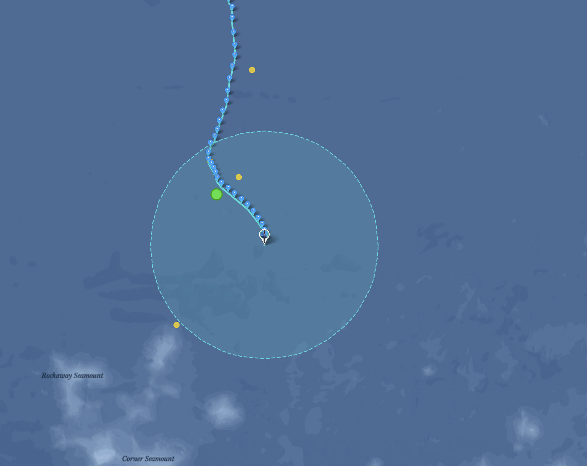
Here’s the forecast he ultimately submitted — run forward from The Monk’s last known position using currents at 700 meters depth, pulled from the Copernicus Marine Service’s Global Ocean Analysis and Forecast product — the Mercator global model.
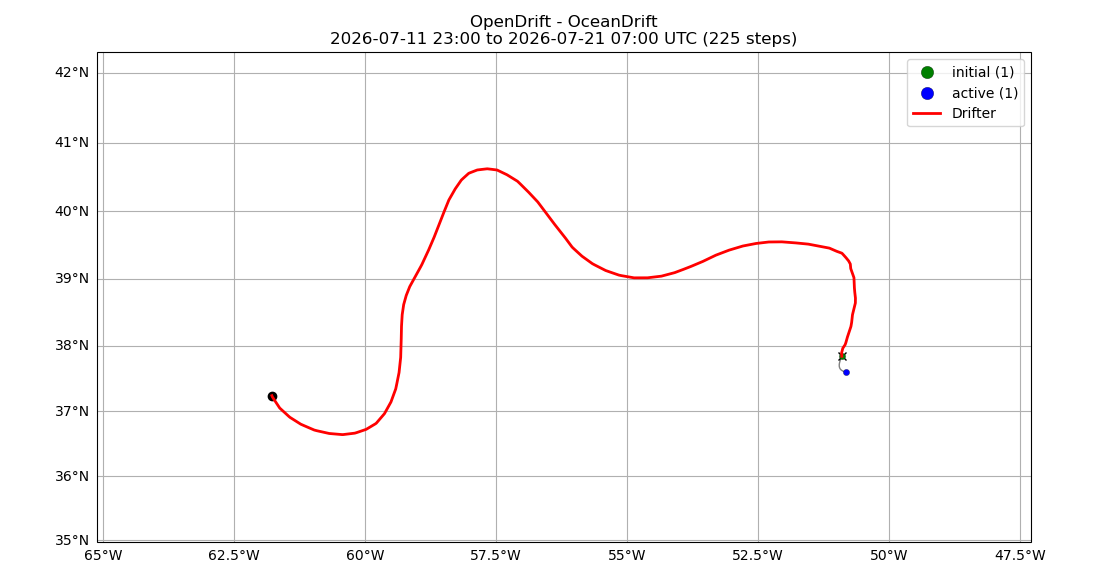
To trust that current field, he tested it against history first. Using the float’s known track from June 1 to July 12, he simulated 24 hours of drift starting from each day’s position, then checked whether the simulated endpoint lined up with where the float actually was the next day.

For comparison, he ran the same test using surface currents instead — checked against the actual track, the surface-current simulations drift visibly off course.

Looked at on their own, without the historical track for reference, those surface-current simulations don’t reveal anything wrong.

But checked the same way against the real track, the 700-meter-depth simulations hug the historical path far more closely — confirming which current field to trust.

“There’s a lot of randomness, a lot of uncertainty in this. It’s like — a dice roll will take it.”
— Knut-Frode Dagestad
This time, the dice landed within 61 km.
04The Interview
What drew you into oceanography in the first place?
“I wanted to study theoretical quantum physics, or something more hardcore physics. But then I found it interesting, though a little far from everyday life — and very narrow. I think it’s nice to do something more related to everyday life, something normal people can relate to.”
“So then meteorology — that was quite interesting. It was actually more mathematical and physical than I expected, because people on the street would say it’s guesswork. They don’t know how much physics is behind meteorology. I liked that it was relevant to society, and still interesting.”
He grew up about an hour inland from Bergen, Norway — near a lake, not the ocean. But I think most people feel attached to the ocean regardless. For me, though, it wasn’t really the ocean itself — it was more the physics, the problem-solving, and a bit of randomness that led me first into meteorology, and then into oceanography, because the two are so connected — you can’t really study one without the other.”
How did OpenDrift come about?
“We already had a service, with some older models running — but we had three different models in three different programming languages. What we realized is there’s so much overlap between oil-spill modeling, search-and-rescue drift modeling, dust modeling, and iceberg modeling that we just made one framework, with separate models for each specific task built on top of it. So we made one generator instead of three separate ones.”
Knut-Frode has worked at MET Norway for about ten or eleven years, building tools for exactly this kind of problem: modeling where things — oil, people and objects in search-and-rescue cases, dust, icebergs — end up carried by ocean currents.
Did you use machine learning for this prediction?
“We do drift modeling with machine-learning corrections at times, but in this case I didn’t use it, because my colleague who works on the machine-learning side was on vacation, and I didn’t want to disturb him. Next time, we’ll add a machine-learning correction to it.”
“I don’t believe in an approach where you use only machine learning. You need a physical grounding as your basis, and you use machine learning as a correction — a post-processing step for the part you can’t otherwise model, the part you can’t fully understand but can fit with machine learning.”
Any advice for people entering the next contest, or using OpenDrift generally?
“I don’t think I’d give advice, because I think it’s good that there’s variability — that people test different approaches. If everyone agreed on the same advice, we’d all end up more uniform, and it might turn out that an approach we didn’t believe in works better. So I wouldn’t give advice — but for my own sake, I believe in a combination of physics as a foundation and a bit of machine learning. Not too much, but a good combination. It’s a fantastic tool — you just have to figure out where to use it and where not to. I think that’s true not just in oceanography, but in society as a whole.”
On the value of the contest format itself:
“I think this competition is not only fun — it’s really useful for everyone involved. It’s a deadline, and you don’t know the answer, so you really need to think and sharpen yourself before submitting. If you’re a researcher just playing with data you already have, you can be focused, but it’s not the same sharpness.”
05What’s Next
There’s more to come — Knut-Frode will be joining us live for “Finding The Monk: How to Predict Where the Ocean Takes a Float,” a walkthrough of the trajectory-prediction techniques behind this win, including the surface-vs-depth validation test and the forecast run above. Bring your questions — he’ll be there to answer them live.
Save the Date
Finding The Monk: How to Predict Where the Ocean Takes a Float
Tuesday, August 18, 2026 · 9:00 AM PDT